87. A Robust LQ Bewley Model#
87.1. Overview#
This lecture embeds the Bewley economy of Consumption Smoothing with Incomplete and Complete Markets in the robust permanent income framework of Robust Consumption Smoothing and Precautionary Savings.
It is the last of four lectures on the LQ permanent income model.
The result is a family of economies in which consumers disagree about the model generating their income, yet behave identically.
Using the observational-equivalence theorem of Hansen et al. [1999], we show
how a continuum of consumers \(i\) can differ in their robustness parameters \(\sigma_i \leq 0\) and their discount factors \(\beta_i\), provided each pair \((\sigma_i,\beta_i)\) lies on an observational-equivalence locus
how every such consumer chooses the same consumption-saving rule as a benchmark \((\sigma = 0, \beta)\) agent who fully trusts the endowment process
how the equilibrium interest rate \(R = \beta^{-1}\) and all aggregate and cross-section dynamics therefore coincide with those of the plain-vanilla Bewley model
how, despite all of this, distinct \((\sigma_i,\beta_i)\) agents hold genuinely different subjective models of their non-financial income
The economy is a pure endowment economy, so there is no physical capital and investment plays no role.
We read Robust Consumption Smoothing and Precautionary Savings as a prerequisite and carry over its notation.
Note
As in Robust Consumption Smoothing and Precautionary Savings, \(w_{t+1}\) is the baseline shock and \(v_{t+1}\) a distortion to its conditional mean, \(\sigma \le 0\) is the robustness parameter, \(\eta_1\) and \(\eta_2\) are the standard deviations of the permanent and transitory endowment shocks, and \(a_t\) denotes net assets.
Let’s begin with some imports.
import numpy as np
import matplotlib.pyplot as plt
87.2. Mapping the Bewley economy into the HST framework#
We specialise the robust model of Robust Consumption Smoothing and Precautionary Savings to \(\lambda = \delta_h = 0\), so there are no habits and no durable goods, and to a pure endowment economy with no physical capital, \(k_t = 0\).
In this case services equal consumption, \(s_t = c_t\).
The only traded security is a one-period risk-free bond, and \(a_t\) denotes the household’s net asset position, so that positive \(a_t\) is wealth.
The endowment process follows the state-space representation
with the two-factor specification \(y_t = z_{1t}+z_{2t}\), \(\check A = \mathrm{diag}(1,0)\) and \(\check C = \mathrm{diag}(\eta_1,\eta_2)\).
The household’s augmented state vector is \(x_t = [a_t,\; z_t^\top]^\top\), and the law of motion of Robust Consumption Smoothing and Precautionary Savings specialises to
The objective is \(\mathbb{E}_0 \sum_{t=0}^\infty \beta^t\bigl[-(c_t - b)^2\bigr]\), which is the HST criterion with \(\sigma = 0\) and a constant bliss level \(b_t \equiv b\).
The period return is written without a factor of \(\tfrac12\), and that choice is not cosmetic: it fixes the scale of the robustness parameter \(\sigma\) used throughout, since rescaling the return rescales \(\sigma\) by the same factor.
The robust Bellman equation with \(\sigma = 0\) therefore reduces exactly to the LQ problem of The LQ Permanent Income Model, confirming that the HST framework nests the Bewley model.
87.3. The robustness scalar for this economy#
Everything about the endowment process that matters for robustness is summarised by the scalar \(\alpha^2\) derived in Robust Consumption Smoothing and Precautionary Savings.
For the two-factor endowment it is
This is the variance of the consumption innovation \(h\,w_{t+1}\), where \(h = (1-\beta)\check G(I-\beta\check A)^{-1}\check C = \begin{pmatrix}\eta_1 & (1-\beta)\eta_2\end{pmatrix}\).
In the present setting \(\alpha^2\) has a second, equally concrete meaning that we met in Consumption Smoothing with Incomplete and Complete Markets.
Because individual consumption is a random walk with innovation variance \(\alpha^2\), the cross-section variance of consumption among agents of age \(t\) who started from a common initial condition is exactly \(t\,\alpha^2\).
So the same scalar that governs how much a consumer’s robustness concern bites also governs how fast the Bewley cross-section fans out.
87.4. The Bewley observational-equivalence locus#
Applying the observational-equivalence theorem Theorem 86.1 of Robust Consumption Smoothing and Precautionary Savings at the equilibrium interest rate \(R = \beta^{-1}\) gives the Bewley observational-equivalence locus
For \(\sigma < 0\) we have \(\hat\beta(\sigma) < \beta\).
An agent with the pair \((\sigma, \hat\beta(\sigma))\) is more concerned about model misspecification, because \(\sigma\) is lower, but also more impatient, because \(\hat\beta\) is lower.
The two forces cancel exactly, leaving the consumption decision rule unchanged.
The locus is admissible only down to the breakdown point of Robust Consumption Smoothing and Precautionary Savings,
Below \(\underline\sigma\) the individual robust control problem has no solution, so there is no economy to describe.
The bound has a transparent reading in terms of the worst-case dynamics derived below.
Since \(\zeta(\sigma) = \beta/\hat\beta(\sigma)\) is the growth rate that agent \(\sigma\) fears for its own marginal utility, the breakdown point is exactly the \(\sigma\) at which
So \(\underline\sigma\) is the robustness level at which the feared growth in marginal utility just reaches the gross interest rate, and the agent’s discounted worst-case objective ceases to converge.
Any stronger concern for robustness would have the agent guarding against a future it cannot value.
87.5. Equilibrium with heterogeneous types#
We can now populate the economy with a continuum of types that differ in their concern for robustness.
Proposition 87.1 (A robust Bewley equilibrium)
Let each agent \(i\) in the unit interval be indexed by a robustness parameter \(\sigma_i \in (\underline\sigma, 0]\), distributed according to any distribution \(\Phi\), and let agent \(i\) have discount factor
so that every pair \((\sigma_i,\beta_i)\) lies on the locus (87.4).
Then
every agent’s optimal consumption plan is identical to that of the plain-vanilla \((\sigma = 0,\, \beta)\) agent,
\(R = \beta^{-1}\) is an equilibrium gross interest rate, independently of \(\Phi\), and
the aggregate and cross-section dynamics coincide with those of the benchmark Bewley economy of Consumption Smoothing with Incomplete and Complete Markets.
Proof. By Theorem 86.1, an agent with parameters \((\sigma_i, \hat\beta(\sigma_i))\) facing gross interest rate \(R = \beta^{-1}\) chooses the same consumption-saving rule as the benchmark \((0,\beta)\) agent.
This holds agent by agent and does not require the \(\sigma_i\) to be equal, which gives part 1.
Since all individual rules coincide with the benchmark rule, the goods-market clearing condition \(\int c_t^i\, di = Y\) and the bond-market condition \(\int a_t^i\, di = 0\) are the benchmark conditions, so they are satisfied at \(R = \beta^{-1}\) for exactly the reason given in Consumption Smoothing with Incomplete and Complete Markets.
Because market clearing never refers to \(\Phi\), neither does the rate that clears the market, which gives part 2.
The argument is a verification: the locus (87.4) is itself constructed at \(R = \beta^{-1}\), so what we have shown is that this rate reproduces itself as an equilibrium for any \(\Phi\), not that no other rate could.
Part 3 follows because aggregate and cross-section objects are integrals of individual paths, and the individual paths are the benchmark paths.
The distribution \(\Phi\) of robustness types is therefore completely unidentified by quantity data.
An econometrician who observes \(\{c_t^i, a_t^i\}\) for every agent and every date cannot tell whether the economy is populated entirely by \(\sigma_i = 0\) agents, entirely by \(\sigma_i\) near \(\underline\sigma\) agents, or by any mixture.
One feature of this equilibrium deserves comment, because it runs against a familiar result.
In a model with heterogeneous discount factors and a common interest rate, the most patient type ordinarily comes to hold all of the wealth, and the long-run distribution degenerates.
Here every type with \(\sigma_i < 0\) has \(\beta_i R < 1\) and so is impatient at the market rate, yet no type decumulates relative to any other.
The reason is that impatience and the precautionary motive are offset at every date, not merely on average, so asset paths as well as consumption paths coincide across types.
Robustness type is therefore uncorrelated with wealth at every horizon, and the usual sorting force is exactly neutralized rather than merely slowed.
87.6. Where the agents genuinely differ#
Agents on the locus are indistinguishable in what they do but not in what they believe.
An agent with \(\sigma_i < 0\) applies a worst-case distortion \(v_{t+1}^i = K(\sigma_i,\beta_i)\,\mu_{s,t}^i\) to its conditional expectations, while an agent with \(\sigma_i = 0\) takes the approximating model at face value.
From Robust Consumption Smoothing and Precautionary Savings, the worst-case law for agent \(i\)’s marginal utility is
with equality only for the fully trusting type \(\sigma_i = 0\).
With \(\lambda = \delta_h = 0\) and a constant bliss point we have \(\mu_{st} = b - c_t\), so agent \(i\)’s worst-case expected consumption path is
Under the approximating model, by contrast, consumption is a martingale, \(\mathbb{E}_t c_{t+h} = c_t\) for every \(h\).
Equation (87.9) says that a robust agent below its bliss point expects, under its worst-case model, that consumption will drift away from bliss at the geometric rate \(\zeta_i\).
The more robust the agent, the faster the drift it guards against, and the more precautionary saving it does.
That extra saving is exactly offset by the lower \(\beta_i\), which is why the realized path is the same for all types.
87.7. Computation#
We use the calibration of the preceding lectures.
β = 0.95        # benchmark discount factor, R = 1/β
η1 = 0.15       # std of permanent shock
η2 = 0.30       # std of transitory shock
b = 1.0         # bliss point

R = 1 / β
h = np.array([η1, (1 - β) * η2])       # consumption innovation loadings
α2 = h @ h
α = np.sqrt(α2)
σ_lo = -(1 - β)**2 / α2                # breakdown point, eq:rbew-breakdown

print(f"α^2 = {α2:.6f}   α = {α:.6f}")
print(f"breakdown σ̲ = {σ_lo:.6f},  where β̂ = {β + σ_lo * α2 * β / (1 - β):.6f}"
      f"  (β² = {β**2:.6f})")
α^2 = 0.022725   α = 0.150748
breakdown σ̲ = -0.110011,  where β̂ = 0.902500  (β² = 0.902500)
Next we build a set of types spread across the admissible range and record what distinguishes them.
We reuse the detection error probability of Robust Consumption Smoothing and Precautionary Savings to report how hard each type’s worst-case model would be to detect in a sample of \(T = 40\) quarters.
def worst_case_persistence(σ, β, α2):
    "Worst-case persistence ζ(σ) of marginal utility, eq:rbew-zeta."
    return 1 / (1 + σ * α2 / (1 - β))


def simulate_paths(ζ, α, T, n_paths, seed):
    "Simulate n_paths draws of μ_{t+1} = ζ μ_t + α w_{t+1} from μ_0 = 0."
    rng = np.random.default_rng(seed)
    paths = np.zeros((n_paths, T + 1))
    shocks = rng.standard_normal((n_paths, T))
    for t in range(T):
        paths[:, t + 1] = ζ * paths[:, t] + α * shocks[:, t]
    return paths


def log_likelihood_ratio(paths, ζ, α):
    "Return log p_worst(path) - log p_approx(path)."
    lag, lead = paths[:, :-1], paths[:, 1:]
    return 0.5 * (np.sum(((lead - lag) / α)**2, axis=1)
                  - np.sum(((lead - ζ * lag) / α)**2, axis=1))


def detection_error_probability(ζ, α, T=40, n_paths=10_000, seed=1234):
    "Finite-sample DEP for the approximating and worst-case scalar laws."
    if np.isclose(ζ, 1.0):
        return 0.5
    approx = simulate_paths(1.0, α, T, n_paths, seed)
    worst = simulate_paths(ζ, α, T, n_paths, seed + 1)
    return 0.5 * (np.mean(log_likelihood_ratio(worst, ζ, α) < 0)
                  + np.mean(log_likelihood_ratio(approx, ζ, α) > 0))
σ_types = np.array([0.0, 0.3, 0.6, 0.9]) * σ_lo
β_types = β + σ_types * α2 * β / (1 - β)
ζ_types = worst_case_persistence(σ_types, β, α2)
dep_types = np.array([detection_error_probability(ζ, α) for ζ in ζ_types])

print(f"{'σ_i':>10}{'β_i':>10}{'ζ_i':>10}{'DEP':>8}")
for σ_i, β_i, ζ_i, dep in zip(σ_types, β_types, ζ_types, dep_types):
    print(f"{σ_i:10.4f}{β_i:10.4f}{ζ_i:10.4f}{dep:8.3f}")
       σ_i       β_i       ζ_i     DEP
   -0.0000    0.9500    1.0000   0.500
   -0.0330    0.9357    1.0152   0.426
   -0.0660    0.9215    1.0309   0.333
   -0.0990    0.9072    1.0471   0.233
These four types differ substantially in patience and in the pessimism of their worst-case model.
We now confirm that they nonetheless behave identically.
Proposition 87.1 asserts that each type, solving its own problem at \((\sigma_i, \beta_i)\), arrives at the benchmark decision rule.
Testing that claim means solving each type’s robust problem separately and comparing the rules that come out.
Assuming the common rule and then reporting that the resulting paths coincide would establish nothing.
We reuse the risk-sensitive LQ solver of Robust Permanent Income and Pricing, renaming its state-cost argument to Rc because \(R\) is the gross interest rate here.
The period return below is \(-(c_t-b)^2\), matching the normalization of \(\sigma\) fixed above.
def solve_rslq(A, B, C, Q, Rc, β, σ, N=None, tol=1e-12, max_iter=50_000):
    "Risk-sensitive LQ regulator; returns F in the rule c = -F x."
    A, B, C, Q, Rc = map(np.atleast_2d, (A, B, C, Q, Rc))
    n, kw = A.shape[0], C.shape[1]
    if N is None:
        N = np.zeros((B.shape[1], n))
    Ω, Iw = -np.eye(n), np.eye(kw)
    for _ in range(max_iter):
        M = Iw - σ * C.T @ Ω @ C
        D = Ω + σ * Ω @ C @ np.linalg.solve(M, C.T @ Ω)
        F = np.linalg.solve(Q - β * B.T @ D @ B, N - β * B.T @ D @ A)
        Acl = A - B @ F
        Ω_new = -Rc - F.T @ Q @ F + (F.T @ N + N.T @ F) + β * Acl.T @ D @ Acl
        if np.max(np.abs(Ω_new - Ω)) < tol:
            return F
        Ω = Ω_new
    raise RuntimeError('risk-sensitive Riccati iteration did not converge')
Write the agent’s problem with state \(x_t = \begin{pmatrix}1 & a_t & z_{1t} & z_{2t}\end{pmatrix}'\) and control \(c_t\), matching the timing of (87.2).
The constant carries the bliss point, and every agent faces the same market rate \(R = \beta^{-1}\); only \(\beta_i\) and \(\sigma_i\) differ across types.
def bewley_lq(b, η1, η2, R):
    "State-space matrices for the agent's problem, period return -(c-b)^2."
    A_x = np.array([[1, 0, 0, 0],
                    [0, R, R, R],
                    [0, 0, 1, 0],
                    [0, 0, 0, 0]], float)
    B_x = np.array([[0.], [-R], [0.], [0.]])
    C_x = np.array([[0, 0], [0, 0], [η1, 0], [0, η2]], float)
    Q_x = np.array([[1.0]])
    Rc_x = np.zeros((4, 4))
    Rc_x[0, 0] = b**2
    N_x = np.array([[-b, 0, 0, 0]], float)
    return A_x, B_x, C_x, Q_x, Rc_x, N_x


A_x, B_x, C_x, Q_x, Rc_x, N_x = bewley_lq(b, η1, η2, R)
F_bench = solve_rslq(A_x, B_x, C_x, Q_x, Rc_x, β, 0.0, N_x)

print("benchmark rule  c = "
      + " + ".join(f"{v:.4f}·{n}" for v, n in
                   zip(-F_bench.ravel(), ["1", "a", "z1", "z2"])))
print(f"implied consumption innovation  {np.round((-F_bench @ C_x).ravel(), 6)}")
print(f"analytic h                      {np.round(h, 6)}")
benchmark rule  c = 0.0000·1 + 0.0500·a + 1.0000·z1 + 0.0500·z2
implied consumption innovation  [0.15  0.015]
analytic h                      [0.15  0.015]
The benchmark rule reproduces the analytic innovation loadings \(h\), which checks that the state-space setup is the one the algebra describes.
Now solve each type’s own problem and compare.
F_types = [solve_rslq(A_x, B_x, C_x, Q_x, Rc_x, β_i, σ_i, N_x)
           for σ_i, β_i in zip(σ_types, β_types)]

print(f"{'σ_i':>10}{'β_i':>10}{'max |F_i - F_bench|':>22}")
for σ_i, β_i, F_i in zip(σ_types, β_types, F_types):
    print(f"{σ_i:10.4f}{β_i:10.4f}{np.max(np.abs(F_i - F_bench)):22.2e}")
       σ_i       β_i   max |F_i - F_bench|
   -0.0000    0.9500              0.00e+00
   -0.0330    0.9357              1.27e-12
   -0.0660    0.9215              2.32e-12
   -0.0990    0.9072              9.43e-12
Every coefficient of every type’s rule agrees with the benchmark to eleven decimal places or better, which is Proposition 87.1 part 1.
To see that this test has power, move each discount factor one percent off the locus, keeping \(\sigma_i\) fixed, and solve again.
print(f"{'σ_i':>10}{'on locus':>12}{'+1% off':>12}{'-1% off':>12}")
for σ_i, β_i in zip(σ_types[1:], β_types[1:]):
    devs = []
    for mult in (1.0, 1.01, 0.99):
        F_off = solve_rslq(A_x, B_x, C_x, Q_x, Rc_x, β_i * mult, σ_i, N_x)
        devs.append(np.max(np.abs(F_off - F_bench)))
    print(f"{σ_i:10.4f}" + "".join(f"{d:12.1e}" for d in devs))
       σ_i    on locus     +1% off     -1% off
   -0.0330     1.3e-12     2.6e-01     2.7e-01
   -0.0660     2.3e-12     4.5e-01     4.7e-01
   -0.0990     9.4e-12     1.7e+00     1.0e+00
A one percent departure from the locus moves the rule in the first decimal place, so the agreement above is not an artifact of the comparison.
Finally, simulate each type using its own solved rule, with common shocks.
T = 60
rng = np.random.default_rng(42)
shocks = rng.standard_normal((T, 2))          # common shocks for all types

c_paths = np.zeros((len(σ_types), T + 1))
for i, F_i in enumerate(F_types):
    x = np.array([1.0, 0.0, 0.0, 0.0])        # [1, a_t, z_1, z_2]
    for t in range(T + 1):
        c_paths[i, t] = -(F_i @ x).item()
        if t < T:
            x = A_x @ x + B_x.ravel() * c_paths[i, t] + C_x @ shocks[t]

print("max absolute difference across types:"
      f" {np.abs(c_paths - c_paths[0]).max():.2e}")
print("max deviation from the random walk with innovation h:"
      f" {np.abs(c_paths[0] - np.concatenate([[0], np.cumsum(shocks @ h)])).max():.2e}")
max absolute difference across types: 1.12e-11
max deviation from the random walk with innovation h: 5.78e-14
The paths coincide, and each reproduces the random walk with innovation \(h\) that the algebra predicts.
The next figure contrasts what the types do with what they believe.
fig, axes = plt.subplots(1, 2, figsize=(11, 4))

for i, σ_i in enumerate(σ_types):
    axes[0].plot(c_paths[i], lw=3 - 0.6 * i, alpha=0.9,
                 label=rf'$\sigma_i={σ_i:.3f}$')
axes[0].set_xlabel('$t$')
axes[0].set_ylabel('$c_t$')
axes[0].set_title('realized consumption')
axes[0].legend()

horizons = np.arange(41)
c_now = c_paths[0, 20]
axes[1].axhline(c_now, color='k', linestyle=':', lw=1.2,
                label='approximating model')
for σ_i, ζ_i in zip(σ_types, ζ_types):
    if σ_i == 0.0:
        continue
    axes[1].plot(horizons, b - ζ_i**horizons * (b - c_now), lw=2,
                 label=rf'worst case, $\sigma_i={σ_i:.3f}$')
axes[1].set_xlabel('horizon $h$')
axes[1].set_ylabel(r'$\hat{\mathbb{E}}_t\,c_{t+h}$')
axes[1].set_title('expected consumption under each belief')
axes[1].legend()

fig.tight_layout()
plt.show()
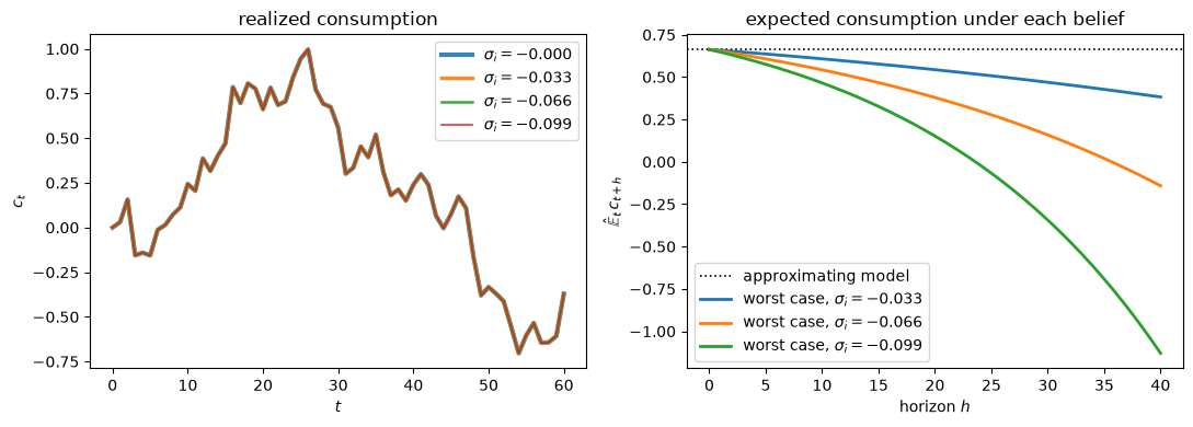
Fig. 87.1 Same actions, different beliefs. Left: realized consumption paths for four robustness types facing common shocks; the curves lie exactly on top of one another. Right: each type’s worst-case expected consumption path from a common date, against the flat martingale forecast of the approximating model.#
The left panel of Fig. 87.1 shows four curves drawn on top of one another.
The right panel shows that the same four agents expect very different futures.
The \(\sigma_i = 0\) agent expects consumption to stay where it is.
Every robust agent guards against a future in which consumption drifts away from the bliss point, and the drift is faster the more robust the agent.
Finally we check part 3 of Proposition 87.1, that the cross-section behaves as in the benchmark Bewley economy.
We simulate a large population spread over the admissible range of types, giving each agent its own shocks and solving each type’s own problem, and compare the cross-section variance of consumption to the benchmark prediction \(t\,\alpha^2\).
n_agents, T_pop = 20_000, 40
rng = np.random.default_rng(1234)

# a population spread over the admissible range, each solving its own problem
σ_pop = np.linspace(0.99 * σ_lo, 0.0, 12)
β_pop = β + σ_pop * α2 * β / (1 - β)
F_pop = [solve_rslq(A_x, B_x, C_x, Q_x, Rc_x, β_j, σ_j, N_x)
         for σ_j, β_j in zip(σ_pop, β_pop)]

type_of = rng.integers(0, len(σ_pop), size=n_agents)
pop_shocks = rng.standard_normal((n_agents, T_pop, 2))
c_pop = np.zeros((n_agents, T_pop + 1))

for j, F_j in enumerate(F_pop):
    m = type_of == j
    x = np.zeros((m.sum(), 4))
    x[:, 0] = 1.0                                    # the constant
    for t in range(T_pop + 1):
        c_pop[m, t] = -(x @ F_j.ravel())
        if t < T_pop:
            x = (x @ A_x.T + np.outer(c_pop[m, t], B_x.ravel())
                 + pop_shocks[m, t] @ C_x.T)

print(f"{'t':>5}{'cross-section var':>20}{'t·α²':>12}")
for t in [10, 20, 30, 40]:
    print(f"{t:5d}{c_pop[:, t].var():20.5f}{t * α2:12.5f}")
print(f"\ncorrelation between σ_i and c_T: "
      f"{np.corrcoef(σ_pop[type_of], c_pop[:, T_pop])[0, 1]:+.4f}")
    t   cross-section var        t·α²
   10             0.22836     0.22725
   20             0.46220     0.45450
   30             0.68968     0.68175
   40             0.91503     0.90900

correlation between σ_i and c_T: -0.0002
The cross-section variance grows linearly at rate \(\alpha^2\), exactly as in Consumption Smoothing with Incomplete and Complete Markets.
Robustness type and consumption are uncorrelated, so the distribution of types leaves no trace in the data even though each agent has genuinely solved a different problem.
87.8. Concluding remarks#
We embedded the single-agent robust permanent income model in a Bewley equilibrium with a continuum of agents who differ in how much they distrust their income process.
Provided each agent’s pair \((\sigma_i,\beta_i)\) lies on the observational-equivalence locus (87.4), every agent chooses the benchmark consumption rule.
The equilibrium interest rate \(R = \beta^{-1}\), the aggregate dynamics, and the linear growth of the cross-section variance of consumption are all inherited unchanged from the plain-vanilla Bewley model of Consumption Smoothing with Incomplete and Complete Markets.
This is a strong non-identification result.
Quantity data pin down the decision rule, but they cannot decompose it into a degree of impatience and a degree of concern about misspecification.
What the agents do not share is their view of the world: each robust type acts as if its consumption were about to drift away from bliss at its own rate \(\zeta_i\).
Two routes lead out of this observational equivalence.
One is to look at asset prices, which do distinguish the \((\sigma,\hat\beta)\) pairs, and which are studied in Robust Permanent Income and Pricing.
The other is to bound the plausible range of \(\sigma\) statistically, using the detection error probabilities of Robust Consumption Smoothing and Precautionary Savings.
87.9. Exercises#
Exercise 87.1
This exercise asks you to carry out the translation from the benchmark Bewley economy into HST notation.
Specialise the robust-control setup to the no-habit, no-capital LQ Bewley environment, so \(\lambda = \delta_h = 0\) and \(k_t = 0\), and let the endowment follow the two-factor model.
Write the household state as \(x_t = [a_t, z_t^\top]^\top\), where \(a_t\) is net assets, and derive the matrices \((A, B, C)\) in (87.2).
Show that when \(\sigma = 0\) the Bellman problem coincides with the LQ permanent-income problem of The LQ Permanent Income Model.
HST define \(\alpha^2 = \nu^\top\nu\) with \(\nu^\top = M_s C\), where \(\mu_{st} = M_s x_t\). Compute \(M_s\) for this economy and verify that this route delivers the same \(\alpha^2\) as (87.3).
Solution
Here is one solution.
With budget law \(a_{t+1} = R(a_t + y_t - c_t)\), \(y_t = \check G z_t\) and \(z_{t+1} = \check A z_t + \check C w_{t+1}\), stacking gives
The sign of \(B\) is negative because higher \(c_t\) reduces asset accumulation.
At \(\sigma = 0\) the minimizing agent is absent, the distortion term drops out of the Bellman equation, and the objective is \(\mathbb{E}_0\sum \beta^t[-(c_t-b)^2]\) subject to a linear law of motion.
That is precisely the LQ permanent-income problem.
With \(\lambda = \delta_h = 0\) and constant bliss, \(\mu_{st} = b - c_t\), and the optimal rule is
so \(M_s = -(1-\beta)\begin{pmatrix}1 & \check G(I-\beta\check A)^{-1}\end{pmatrix}\) up to the constant.
Since \(C = [0;\ \check C]\), the first column of \(M_s\) is annihilated and
Hence \(\alpha^2 = \nu^\top\nu = hh^\top = \eta_1^2 + (1-\beta)^2\eta_2^2\), matching (87.3).
The minus sign is immaterial because only \(\alpha^2\) appears.
Exercise 87.2
This exercise works through the equilibrium logic of Proposition 87.1.
Fix a benchmark pair \((\beta, \sigma = 0)\) with \(R = \beta^{-1}\) and let a unit interval of consumers be indexed by \(i\), with type \(\sigma_i \in (\underline\sigma, 0]\) and discount factor \(\beta_i = \hat\beta(\sigma_i)\) from (87.4).
Use Theorem 86.1 of Robust Consumption Smoothing and Precautionary Savings to show that each type has the same consumption rule as the benchmark \((\beta, 0)\) agent.
Show that goods- and bond-market clearing imply the same equilibrium interest rate \(R = \beta^{-1}\) as in the plain-vanilla Bewley model, whatever the distribution of types.
Explain why agents can be observationally equivalent in quantities while holding different worst-case subjective models.
Suppose instead that agents share a common \(\beta\) but differ in \(\sigma_i\), so that they are not on the locus. Explain why \(R = \beta^{-1}\) would then generally fail to clear the bond market.
Solution
Here is one solution.
Theorem 86.1 says that if \((\sigma_i,\beta_i)\) satisfies \(\beta_i = \beta + \sigma_i\alpha^2\beta/(1-\beta)\), then type \(i\) chooses the same decision rule as the benchmark agent, so all types share the policy function \(c_t = \mathcal{C}(a_t, z_t)\).
Since all individual rules coincide with the benchmark rule, aggregating over \(i\) reproduces the benchmark market-clearing conditions, which hold at \(R = \beta^{-1}\).
The type distribution never enters, so it cannot affect the equilibrium rate.
Observational equivalence is a statement about quantities generated by optimal rules.
The minimizing feedback \(K(\sigma_i,\beta_i)\) still differs across types, so the agents attach different worst-case conditional means to the same shock process while making identical choices.
Off the locus the impatience offset is missing.
An agent with \(\sigma_i < 0\) and discount factor \(\beta\) has a precautionary motive that is not cancelled, so it wants to save more than the benchmark agent at \(R = \beta^{-1}\).
With positive net demand for bonds in the aggregate, the equilibrium interest rate must fall below \(\beta^{-1}\) to clear the market, and the equilibrium then depends on the whole distribution of types.
Exercise 87.3
This exercise separates quantities from beliefs for two individual agents.
Consider agents \(a\) and \(b\) with \(\sigma^a < \sigma^b \leq 0\), both on the locus (87.4).
Show that the two agents have the same consumption innovation \(h\,w_{t+1}\).
Show that if they start from the same \((a_t, z_t)\) and observe the same shock \(w_{t+1}\), their next-period consumption and assets coincide.
Using (87.9), compute the ratio of the two agents’ worst-case forecasts of \(b - c_{t+h}\) and show that it grows geometrically in \(h\).
Summarise what is and is not identified by data on quantities alone.
Solution
Here is one solution.
Both pairs lie on (87.4), so by Theorem 86.1 both use the benchmark rule and hence the same innovation vector \(h\).
With a common state and a common shock, both agents apply the same policy function and the same law of motion, so \(c_{t+1}^a = c_{t+1}^b\) and \(a_{t+1}^a = a_{t+1}^b\).
From (87.9), \(\hat{\mathbb{E}}_t (b - c_{t+h}^j) = \zeta_j^{\,h}(b-c_t)\), so the ratio is \((\zeta_a/\zeta_b)^h\).
Since \(\sigma^a < \sigma^b\) implies \(\zeta_a > \zeta_b\), the ratio grows geometrically: the two agents’ beliefs diverge without bound as the horizon lengthens, even though their actions never differ at all.
Quantities identify the equilibrium decision rule, and hence the single combination of parameters that appears in it.
They do not identify the decomposition of that rule into impatience \(\beta_i\) and robustness \(\sigma_i\) along the locus.
Exercise 87.4
This exercise asks how much belief heterogeneity is statistically plausible.
Restrict attention to types whose worst-case model has a detection error probability of at least \(0.25\) in a sample of \(T = 40\).
Find the most robust admissible type \(\sigma^{\min}\) by bisection.
For that type, report \(\beta_i\), \(\zeta_i\), and the horizon \(h\) at which its worst-case forecast of \(b - c_{t+h}\) is twice the approximating model’s forecast.
Repeat part 1 with \(T = 160\) and comment on what a longer sample does to the plausible amount of belief heterogeneity.
Solution
Here is one solution.
The approximating model forecasts \(b - c_{t+h} = b - c_t\) for every \(h\), while the worst-case forecast is \(\zeta_i^h(b-c_t)\), so the doubling horizon solves \(\zeta_i^h = 2\).
def σ_for_target_dep(target, T, β, α2, tol=1e-5):
    """
    Find σ ∈ (σ̲, 0) with DEP(σ) = target by bisection.

    Returns None if the DEP never falls to the target on the admissible
    range, in which case the breakdown point is the binding constraint.
    """
    α_loc = np.sqrt(α2)
    lo, hi = 0.999 * (-(1 - β)**2 / α2), 0.0

    def dep_at(σ):
        return detection_error_probability(
            worst_case_persistence(σ, β, α2), α_loc, T=T)

    if dep_at(lo) > target:
        return None

    while hi - lo > tol:
        mid = 0.5 * (lo + hi)
        if dep_at(mid) < target:
            lo = mid
        else:
            hi = mid
    return 0.5 * (lo + hi)


for T in [40, 160]:
    σ_min = σ_for_target_dep(0.25, T, β, α2)
    if σ_min is None:
        σ_min = 0.999 * σ_lo        # breakdown binds before detectability
        note = ' (breakdown point binds)'
    else:
        note = ''
    ζ_min = worst_case_persistence(σ_min, β, α2)
    print(f"T = {T:>3}:  σ_min = {σ_min:.5f}   β_i = {β / ζ_min:.5f}   "
          f"ζ_i = {ζ_min:.5f}   doubling horizon = "
          f"{np.log(2) / np.log(ζ_min):.1f} quarters{note}")
T =  40:  σ_min = -0.09313   β_i = 0.90979   ζ_i = 1.04420   doubling horizon = 16.0 quarters
T = 160:  σ_min = -0.02322   β_i = 0.93997   ζ_i = 1.01067   doubling horizon = 65.3 quarters
At \(T = 40\) statistical detectability binds before the breakdown point does, so the most robust plausible type is interior.
At \(T = 160\) it binds far sooner and the plausible set of types shrinks sharply toward \(\sigma = 0\).
The doubling horizon lengthens correspondingly: with more data, only agents whose pessimism accumulates slowly remain statistically credible.
Note
The detection error probability is estimated by simulation, so a target close to the value attained at \(\underline\sigma\) makes the answer sensitive to the random seed.
At \(T = 40\) the DEP at the breakdown point is almost exactly \(0.2\), which is why the target here is \(0.25\).